Digital face manipulation has applications in many domains including the film industry. For example, a stuntman can be recorded while performing in action scenes and afterwards the face of the movie star can be realistically transferred to that footage to trick the viewer into thinking that he was watching the actor the whole time. In previous decades, it required hours of post-editing, but now thanks to advances in computer vision it can be applied with a single click.

More formally, the goal of face swapping is to take the face from source image and paste it into the target image. The output should be an image with background of the target seamlessly blended with the face identity of source.

Face swapping is a complex task that can be broken down into the following steps: face detection on both images, transferring the source face in the correct pose and expression in the target image and face blending, i.e. adjusting the lighting, skin tone etc. In this project, we used a pretrained network $f_{det}$ for face detection using facial landmarks and focused on the other parts of this process.

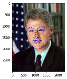
Facial landmarks are points that outline important regions present in every face, such as eyes, mouth, chin etc. In the picture below the detected facial landmarks are depicted in blue.

We compare 3 algorithms with qualitative and quantitative results:

Naive approach
Optimization-based approach
GAN-based approach

Naive approach

In this case, we detect the face in source image and apply it directly on the target without any adjustments.

Optimization-based approach

This approach represents classical computer vision methods before the deep learning era. The main improvement is that it estimates the pose and expression in the target image and applies it to the source face to produce the final image.

Before getting into face swapping, let’s first consider how to estimate the pose. Imagine we have two 2D images, $I_1$ and $I_2$ with the same face but different poses and expressions. On a high-level, this can be done like so:

Build a 3D model $G_1$ of the face in $I_1$ .
Transform $G_1$ into $\hat{G}_1$ : $\hat{G_1}=G_1R^T+t$ where $R$ is a rotation matrix and $t$ is translation vector.
Project $\hat{G}$ back into a 2D image $I'_1$ .
Find $R$ and $t$ by optimizing the difference between $I'_1$ and $I_2$ .

In detail, this translates to:

We need to use a compact face representation in order to limit the search space for $R$ and $t$ . This is done with a PCA model. Therefore, first extract 3D landmarks from the $I_1$ with $f_{det}$ and then build a 3D face representation $G$ parametrized by $\alpha$ and $\delta$ of the input face with $f_{PCA}$ .
Transform $G$ into $\hat{G}$ : $\hat{G}=GR^T+t$ where $R$ is a rotation matrix and $t$ is translation vector.
Project $\hat{G}$ back into 2D, assuming a pinhole camera model $\Pi$ .
Find $\alpha$ , $\delta$ , $R$ and $t$ using energy optimization.

For face swapping with source image $I_s$ and target image $I_t$ the pipeline is:

Perform the procedure above for both images to find $\alpha_s$ , $\delta_s$ , $R_s$ , $t_s$ and $\alpha_t$ , $\delta_t$ , $R_t$ and $t_t$ .
Transform the 3D face representation of source image $G(\alpha_t, \delta_s)$ according to the pose of target image $R_t$ and $t_t$ : $\hat{G}= G(\alpha_t, \delta_s)R_t^T+t_t$ .
Project $\hat{G}$ into 2D, assuming a pinhole camera model $\Pi$ , interpolate to fill missing pixels.
Render the projection on the target image.

One of the main issues of this method is that new $\alpha$ , $\delta$ , $R$ and $t$ have to be learnt from scratch for every image which vastly increases face swapping time for every pair. As we will see in later sections, the face swapping quality is also quite poor.

GAN-based approach

Generative Adversarial Networks

Generative Adversarial Networks (GANs) were initially proposed for simple image generation and achieved more realistic outcomes than other methods such as variational autoencoders or normalizing flows. They consist of two networks. The generator network $G$ tries to generate realistic fake image $G(z)$ while the discriminator $D$ tries to detect if an image is real or created by the generator. The generator aims to fool the discriminator which leads to increasingly high quality images.

Formally, discriminator loss is:

$\mathcal{L}_{D}=\mathbb{E}_{x \sim X}[-\log D(x)]+\mathbb{E}_z[-\log (1-D(G(z)))]$

where:

$x$ is a real image sample from the real data distribution $X$
$z$ is a random sample from a normal distribution, which serves as a random seed for the generator
$\mathbb{E}$ as usual denotes the expectation

On the other hand, the generator loss is:

$\mathcal{L}_{G}=-\mathcal{L}_{D}=\mathbb{E}_z[-\log (1-D(G(z)))]$

FSGAN

Multiple papers extended this technique to face blending, including FSGAN which we partially re-implemented in this project. This paper proposes a whole pipeline with 4 different generators for face reenactment $G_r$ , segmentation of face and hair $G_s$ , face inpainting $G_c$ and finally blending $G_b.$ Due to time constraints, we only focus on the blending part (in yellow in the diagram before).

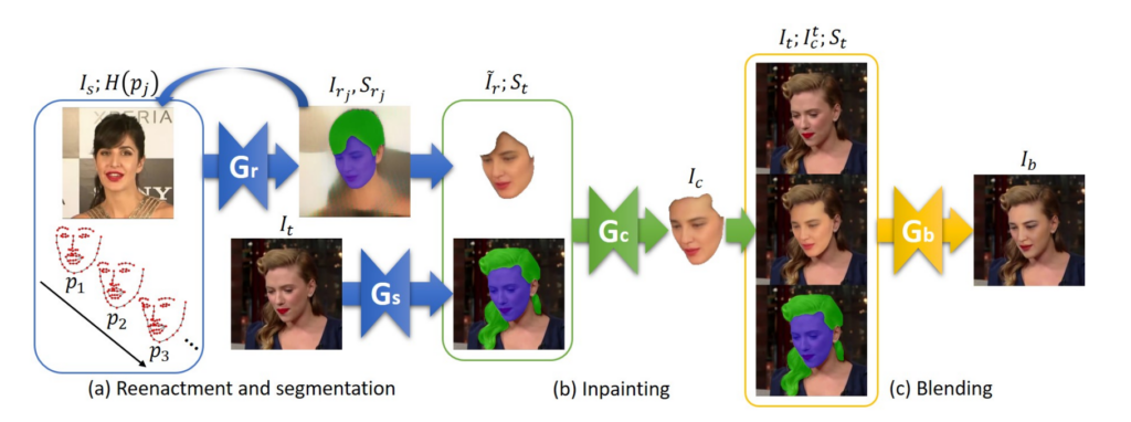
The input of the blending generator $G_b$ is the target image $I_t$ , the target image overlaid with the pose-aligned source face $I_c^t$ and the face segmentation mask $S_t$ of the target. The networks outputs the blended image $I_b$ .

We use a multi-scale generator based on ResUnet and a multi-scale discriminator based on Pix2PixHD consisting of multiple discriminators, $D_1, D_2, ..., D_n$ , each one operating on a different image resolution.

Losses

Imagine you have to teach someone to judge if a pair of images is blended well. How would you describe it to a person that has never seen a page? Measuring face blending quality is difficult to express explicitly and therefore the authors use a combination of multiple losses that optimize different criteria.

The perceptual loss $\mathcal{L}_{perc}$ , aims to make image representations (of a pretrained model) of the blended image as similar as possible to image representations of the ground truth. This encourages the network to focus on high-level image features instead of values on particular pixel values. The authors pretrain a VGG-19 network on face recognition and face attribute classification task which can extract image representation from input images. Let $F_i \in \mathbb{R}^{C_i \times H_i \times W_i}$ be the feature map of the i-th layer of the network. Let $x$ be the predicted output and $y$ be the ground truth (for now these two variables might seem a bit abstract, but in a couple paragraphs we will replace $x$ and $y$ with more concrete variables specific to this setup). The perceptual loss is given by:

$\mathcal{L}_{\text {perc }}(x, y)=\sum_{i=1}^n \frac{1}{C_i H_i W_i}\left\|F_i(x)-F_i(y)\right\|_1$

The perceptual loss on its own does not perform well on its own, so additionally a pixel-wise L1 loss $\mathcal{L}_{\text {pixel }}$ is implemented which regresses the exact pixel values.

$\mathcal{L}_{\text {pixel }}(x, y)=\|x-y\|_1$

These two compliment each other and their weighted sum is the reconstruction loss $\mathcal{L}_{rec}$ :

$\mathcal{L}_{\text {rec }}(x, y)=\lambda_{\text {perc }} \mathcal{L}_{\text {perc }}(x, y)+\lambda_{\text {pixel }} \mathcal{L}_{\text {pixel }}(x, y)$

Next, we need a variation of the loss used in the original GANs. As discussed in the previous section, the discriminator $D$ actually consists of $n$ discriminators $D_1, ..., D_n$ applied to different image scales. The adversarial loss $\mathcal{L}_{adv}$ is:

$\mathcal{L}_{a d v}=- \sum_{i=1}^n \mathcal{L}_{D_i}$

where $L_{D_i}$ is the discriminator loss that we already mentioned above:

$\mathcal{L}_{D_i}=\mathbb{E}_{x \sim X}[-\log D_i(x)]+\mathbb{E}_z[-\log (1-D_i(G(z)))]$

Finally, we obtain the blending generator loss $\mathcal{L}_{G_b}$

$\mathcal{L}_{G_b}=\lambda_{\text {rec }} \mathcal{L}_{r e c}(x,y)+\lambda_{a d v} \mathcal{L}_{adv}$

Before we defined $x$ and $y$ as the predicted output and the ground truth and decided to worry about them later. In our case, $x$ is the blended image $I_b$ returned by the generator. However, there is no real ground truth to use. Therefore, the authors create the ground truth with Poisson blending optimization. It is a common technique used in image editing and implemented in OpenCV. It might be unclear why train a model to approximate some optimization technique instead of just using the technique itself for blending. However, we will show that FSGAN’s blending quality vastly improves upon Poisson blending. On top of that, for Poisson blending, the optimization problem have to be solved separately for every image which increases inference time. In summary, we can replace $y$ with an image created with Poisson optimization $I_p$ .

$\mathcal{L}_{G_b}=\lambda_{\text {rec }} \mathcal{L}_{r e c}\left(I_b, I_p\right)+\lambda_{a d v} \mathcal{L}_{adv}$

This is what the authors call the Poisson blending loss.

Qualitative results

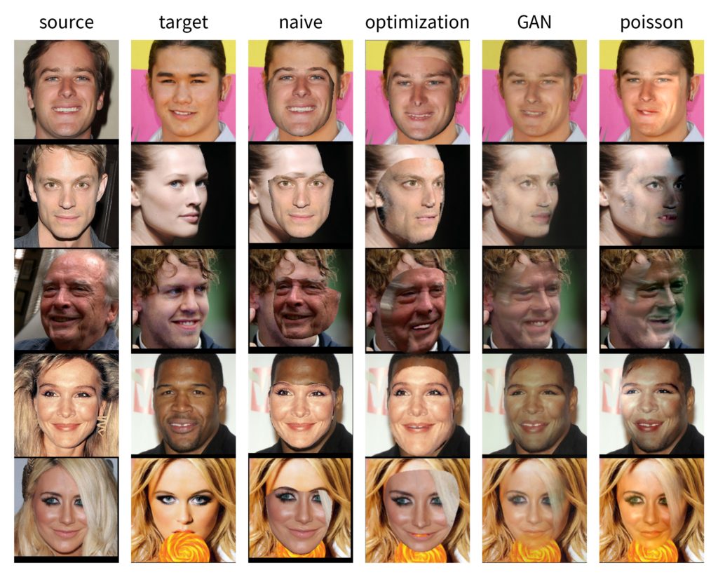
Above we show qualitative results for all approaches. Each row contains a different image pair and each column contains a different baseline or approach. We carefully selected this group of images to focus on the strengths and weakness of examined approaches. From left to light we show: source image, target image, naive approach, optimization-based approach, GAN approach and ground truth (poisson blending) used for GAN training. The first image is an easy example where both faces have similar skin color and angle, there is no hair occlusion and the lighting is similar. The second and the third pair contains faces with a large variation in pose on a dark background and with varying backgrounds. The second last image pair shows how the algorithms handle varying sking color and the last displays the ability of presented approaches to handle hair or object occlusions (in this particular case the lollipop is occluding the chin and the lower lip).

The naive approach (third column) looks very artificial in all images. For easy examples it at least overlaps with the target face while for pairs with varying pose it fails completely. Optimization-based method adjusts the pose well for easier images, but leaves room for improvement especially when the pose is very different between source and target image. Finally, the GAN approach obtains the best results. It is especially impressive in cases with variation of pose (second and third rows) – at the edge between the face and the background, the ground truth gradually blends one into another while GAN makes a sharp line in between them which looks much more realistic. It also obtains the best results in the forth row by producing quite a natural image from a pair with drastically different skin tones. Unfortunately, all of the methods struggle with occlusions as presented in the last row, although even then GAN-based approach seems superior as the hair is more transparent in its outputs. This defect could be clearly improved by additionally segmenting hair and face as part of the full FSGAN pipeline.

Quantitative results

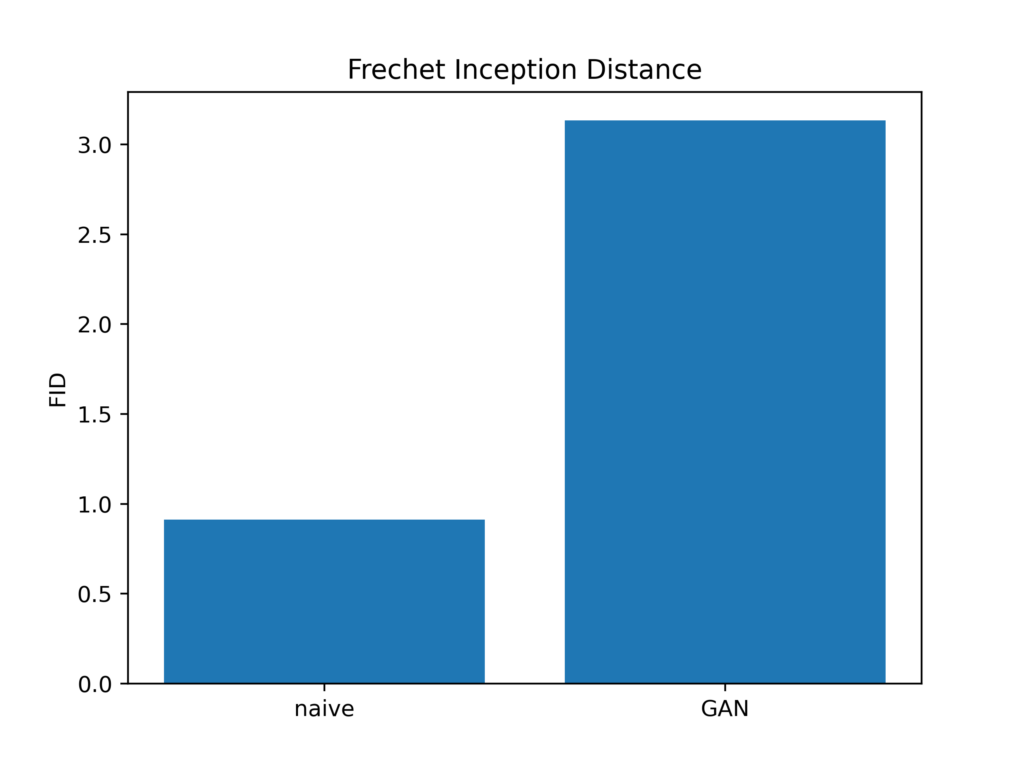
While qualitative inspection of generated images does show to some extent the quality of various algorithms, it has a number of drawbacks, e.g. when considering two similarly performing algorithms it is not possible to definitively determine which one is better or the presented results might be cherry-picked. Quantitative metrics usually mitigate those issue, but in the case of generative adversarial networks there is no ground truth and therefore there is no straightforward manner to compute such metrics. To make matters worse, there are no established metrics for face blending. The most common measures for image generation are the Inception Score and Frechet Inception Distance. The Inception Score is performed by feeding a generated image through the Inception model and is based on two assumptions – conditional class probabilities on ImageNet should have high entropy (there should be only a few classes with high probability) and the model should produce diverse images. These two goals are optimized with Inception Score. This approach has multiple drawbacks such as excessive sensitivity to weights and inadequacy for dataset other than ImageNet. On the other hand, Frechet Inception Distance compares the distribution of real and fake images using the first two moments – mean and standard deviation. We use the source images as the real image because they contain the transferred face which is the most important part of face swapping.

As shown in the bar plot, FID yields opposite results to our qualitative observations – the best FID is obtain by the naive approach and the worst by the GAN-based approach. This confirms the limitations we mentioned because both FID and IS are designed to be used for evaluating GANs in the classic task of generating reliable images while our use case, blending two real faces, is quite different and renders those metrics hardly useful.

Błażej Dolicki

Face swapping with GANs

Naive approach

Optimization-based approach

GAN-based approach

Generative Adversarial Networks

FSGAN

Losses

Qualitative results

Quantitative results

Like this:

Leave a Reply Cancel reply

Naive approach

Optimization-based approach

GAN-based approach

Generative Adversarial Networks

FSGAN

Losses

Qualitative results

Quantitative results

Share this:

Like this:

Leave a Reply Cancel reply